Excel percentage formulas: 6 general uses

Desk of Contents

Show Extra

Excel percentage formulas can safe you through complications stout and puny every single day—from determining gross sales tax (and pointers) to calculating increases and decreases. We’ll crawl through several examples below: turning fractions to percentages; backing gross sales tax out of totals; percentage of total; percentage raise or decrease; percentage crowning glory; and p.c ranking (percentile).

Straightforward how to relate fractions into percentages

Percentages are a fragment (or half) of 100. The mathematics to establish a percentage is to divide the numerator (the number on high of the half) by the denominator (the number on the bottom of the half), then multiply the answer by 100. As an illustration, the half 6/12 turns staunch into a decimal fancy this: 6 divided by 12 (which equals 0.5) times 100 equals 50 p.c.

In Excel, you don’t desire a method to remodel a half to a p.c—appropriate a Format alternate. As an illustration:

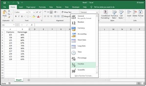
1. Enter 10 fractions in column A (from A2 through A11). (Show: Excel mechanically reduces fractions to their lowest phrases, corresponding to fixing 6/10 to three/5.)

Since the Excel default is decimal, you’ll want to spotlight the differ and layout it for Fractions. Here’s how:

2. Reproduction the fractions in column A to Column B.

3. Highlight that differ and lumber to the Dwelling tab. Preserve Share from the dropdown list in the Quantity Formats subject.

JD Sartain / IDG

NOTE: It’s possible you’ll presumably well presumably furthermore seize out Format Cells from the Format button in the Cells neighborhood.

Straightforward how to support gross sales tax out of totals

Some firms sell products with the gross sales tax incorporated, then appropriate support the tax out for his or her funds to the IRS. Calculate this by dividing the “sticker” designate (or receipt total) by 1.0 plus the gross sales tax price. As an illustration, if you paid $50 for a lamp and the local gross sales tax price is 9%, divide $50 by 1.09. The precise retail designate before gross sales tax is $45.87, and the gross sales tax is $4.13. To ascertain your answer, appropriate add the 2 numbers collectively, or multiply $45.87 by 9%.

Using a calculator to create this for appropriate one item is handsome, nevertheless if you’re pulling gross sales taxes out of your weekly or month-to-month product gross sales, you most fascinating want to enter the method once, then reproduction it for the length of your entire gross sales and stock spreadsheet.

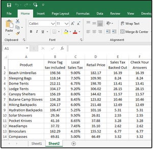
1. Enter a dozen or so products in column A (from A2 through A14).

2. Subsequent, enter the corresponding receipt total designate (tax incorporated) in column B (from B2 through B14).

3. In columns C2 through C14, enter several arbitrary gross sales tax percentages (so you may possibly well bear some fairly about a numbers to play with). Originate obvious to enter some decimal/fractional percentages corresponding to 4.75%, as a result of most gross sales taxes must not entire numbers.

4. Enter this two-step method in cell D2: =SUM(B2/(C2+1)) . The object right here is to remodel the tax percentage to the entire number divisor (e.g., 9% to 1.09), after which divide the receipt total designate ($198.56) by the entire number divisor (1.09) to safe the handsome retail designate (before taxes) of $182.17.

5. Reproduction the method from D2 all of the manner down to D14.

6. In cell E2, subtract D2 from B2 to safe the precise “backed-out” gross sales taxes (for the IRS): =SUM(B2-D2). Reproduction the method from E2 down through E14.

7. To double-verify your solutions, enter this method in F2 through F14: =SUM(D2*C2). If the columns E and F match, your files is handsome.

JD Sartain / IDG

Straightforward how to safe percentage of totals

Whenever you’re self-employed or bear an position of enterprise on your property, one diagram the IRS uses to establish your deductions (for the position of enterprise fragment of your rent, utilities, household upkeep costs, etc.) is to subtract the square pictures of the position of enterprise from the residence’s total square pictures. It’s possible you’ll presumably well presumably teach a percentage of those totals. The mathematics for this one begins with dividing the position of enterprise square pictures by the residence’s total square pictures, then calculating the overhead in line with that percentage.

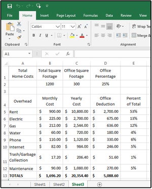
1. Across the head, enter your property’s total square pictures in cell B2.

2. Enter the final square pictures of your position of enterprise in C2.

3. Enter this method in cell D2: =SUM(C2/B2) to establish the position of enterprise’s percentage of square feet (on this case, 25%).

4. Enter your property and position of enterprise overhead objects in column A (rent, electrical energy, etc.)

5. Enter the month-to-month designate of every item in column B.

6. Enter this method in cells C5 through C12: =SUM(B5*12) . This supplies you the yearly totals.

7. Enter this method in cells D5 through D12: =SUM(C5*$D$2). The cell handle D2 want to be absolute. Employ characteristic key F4 so to add the dollar indicators that accomplish the method absolute, so every cell in column D is multiplied by D2.

8. Complete columns B, C, and D on row 13.

Now you may possibly well look for how powerful you spent on month-to-month and yearly overhead for the final house and for the position of enterprise most fascinating. Cell D13 reveals your total residence position of enterprise deduction ($5,088.60).

9. To calculate the p.c of the final overhead by item, enter this method in E5 through E12: =SUM(B5/$B$13). Employ these percentages to establish if your month-to-month/yearly overhead is within same old enterprise practices.

JD Sartain / IDG

Share of totals for residence position of enterprise deduction and overhead

Straightforward how to identify percentage of designate raise or decrease

For deal of firms, critically in retail, owners and managers attach finish to know the percentages of raise and decrease for appropriate about every little thing, from gross sales to salaries. Employ the following formulas to calculate the percentages of raise and decrease on your firm.

Have faith in you’ve created a workbook with a spreadsheet tab called “Amplify-Lower.” Every other spreadsheet tab called “SalesTax” entails Retail Sales Label files.

1. Enter a dozen or so product objects in column A of Amplify-Lower (or appropriate reproduction the same objects gentle in the spreadsheet from fragment A above).

2. Enter the portions supplied of every item in columns B and D.

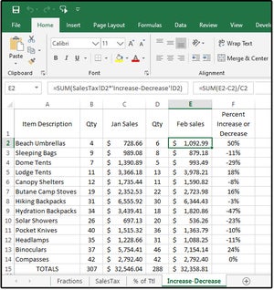
3. Enter this method in the “Jan Sales” column (C2 through C14): =SUM(SalesTax!D2*’Amplify-Lower’!B2). This method tells Excel to multiply the Retail Sales Label in column D of the spreadsheet called SalesTax by the amount amounts in column B of the spreadsheet where our cursor for the time being resides, Amplify-Lower.

4. Enter this method in the “Feb Sales” column (E2 through E14): =SUM(SalesTax!D2*’Amplify-Lower’!D2).

5. Subsequent, enter this method in F2: =SUM(E2-C2)/C2.

The horrible numbers expose the gross sales raise percentage between January and February, whereas the detrimental numbers signify the proportion of decrease in gross sales.

JD Sartain / IDG

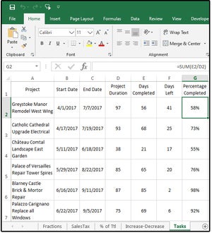
Straightforward how to calculate percentage of a process or project completion

As an different of spending cash on a project management pc tool, use the following formulas to attach watch over the planning and drift of every project with the proportion crowning glory at specified intervals.

1. In column A, enter the names for half a dozen initiatives (in development).

2. In columns B and C, enter the Start and Discontinuance Dates of every project.

3. To uncover the project completion (prior to now), subtract the Start Date from the Discontinuance Date. Enter this method in column D2 through D7: =SUM(C2-B2).

4. In column E, enter the selection of days performed prior to now. Here’s the most fascinating column of files that you may possibly well presumably well ever alternate; as an instance, once a day (or week), safe entry to this spreadsheet and modify the guidelines on this column to safe appropriate form conclusions in columns F and G (days left and percentage performed).

5. To safe the selection of days left in every project, enter this method in column F2 through F7: =SUM(D2-E2). This numbers will constantly alternate in line with the number files in column E (choice of days performed).

6. And final, enter this method to safe the proportion of the duty/project performed, prior to now: =SUM(E2/D2).

JD Sartain / IDG

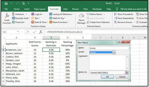
Straightforward how to create p.c ranking

Have faith in you may possibly well bear dozens of people making use of for nationwide parks and forestry jobs. From the resumes and the initial interviews, they all appear to be equally licensed. Then all once more, they must meet some minimal expertise which can presumably well be not customarily indicated on resumes, such because the staunch approach to safely identify porcupine quills from a dogs’s face and neck.

The answer: Give the candidates a expertise test, and use Excel’s PERCENTRANK.EXC characteristic to establish the ranking percentile of every applicant.

Enter 10 applicant names in cells A2:A11. Enter the skill components (ratings) between 10 and 100 for every applicant in cells B2:B11 after which title the differ.

Preserve/spotlight cells B2:B11. Preserve Formulation > Outline Title > Outline Title and enter the note Ratings in the Title subject box. Click the arrow beside the Scope subject box and procure Sheet1 from the list to title the differ position. Search the Refers To subject box contains the cell addresses of the highlighted/selected differ. If the differ is unsuitable, click on the pink arrow on the staunch and enter the handsome differ addresses, or re-seize out the handsome cells, after which click on OK.

NOTE: You will want outline and title the differ of the “array” for the method to work.

Subsequent, enter the following method in cell C2: =PERCENTRANK.EXC(Ratings,B2,2) where Ratings equals the differ title, B2 is the first designate in the differ, and 2 diagram camouflage two decimal locations.

Reproduction and paste the method down through cell C11. Search that the most fascinating portion of the characteristic that adjustments as you cursor down through list is the cell handle (B2, B3, B4, etc.).

It’s possible you’ll presumably well presumably layout the decimal numbers as a p.c for simpler viewing. Actual spotlight the differ and seize out P.c from the Format Cells dialog. Or Reproduction column C and  procure Paste > Particular > Values to replicate the text in column D. Show, nevertheless, that if you alternate any of the values in column B, you must repeat the Reproduction-Paste-Particular-Values step.

To ensure that the values are frequently updated and contemporary, enter the following method in D2: =VALUE(C2), then reproduction and paste down through D11.

Search that three candidates bear 22 components with a ranking percentile of 72 p.c. This fashion that their ratings are larger than or equal to 72 p.c of all of the test ratings. Whenever you alternate the first salvage from 22 to 23, the ranking percentage jumps to 90 p.c, as a result of this salvage is now in the head 90th percentile of all of the test ratings.

JD Sartain / IDG

JD Sartain is a technology journalist from Boston. She writes the Max Productivity column for PCWorld, a month-to-month column for CIO, and atypical characteristic articles for Network World.